Connective Field (CF) modeling extends the classical concept of the receptive field, which is the portion of sensory space that elicits responses when stimulated. That is, the receptive field model describes a function that relates a stimulus to a response. The twist of CF modeling is that it defines this response function in terms of brain activations instead of stimulus parameters: it’s a brain-to-brain model that explains brain responses from other brain responses. The linear CF model explains responses throughout the brain in terms of the spatial pattern of activation on the surface of a topographic brain region.

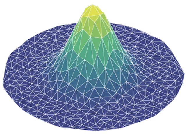
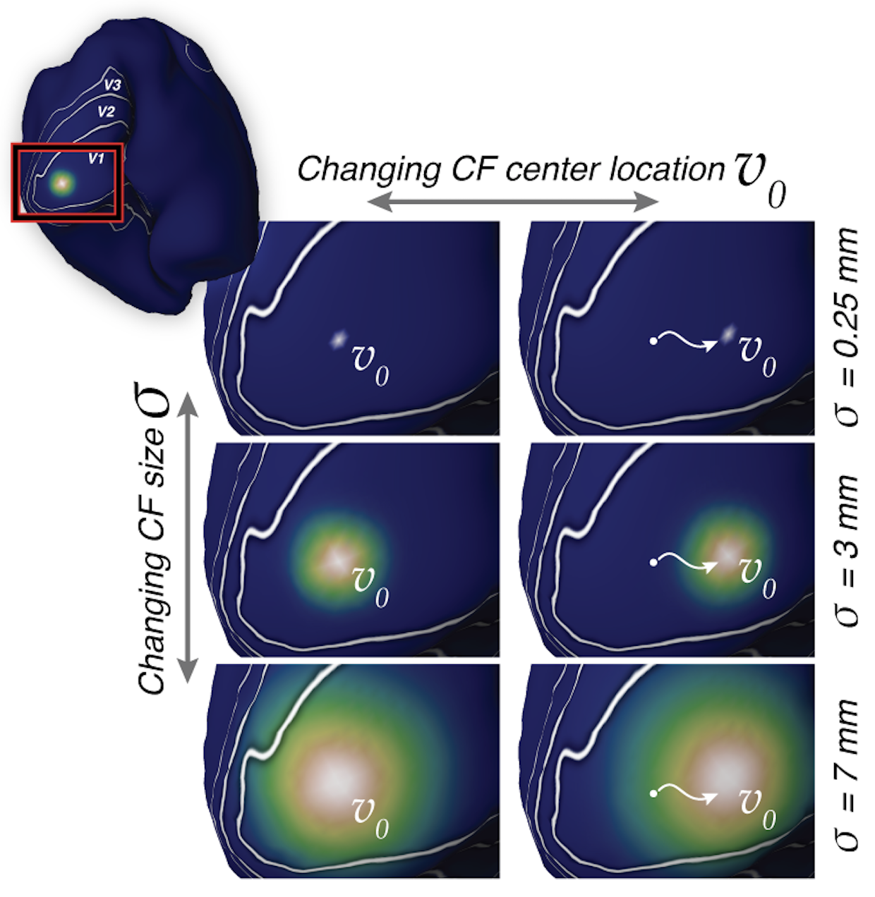Specifically, brain responses are modeled as relating to a Gaussian region on the surface, providing several biologically relevant quantifications. Depending on the source region, the location of the peak of the Gaussian region (the first parameter of the CF model) represents a location in visual space, a frequency of sound, or an impression of touch somewhere on the body. That is, the CF model uses sensory topographies to translate brain activations into sensory impressions. Its standard deviation (size, the second parameter of the CF model), expressed in the physical unit of mm on the cortical surface, represents the scale of information integration in the relevant sensory modality.

The practical power of this computational model is two-fold: First, because CF modelling is based only on brain activations, its parameters can be estimated from the data of any neuroimaging experiment. Second, the model parameters are biologically interpretable, making them relevant for computational theory – as well as possibly clinically relevant.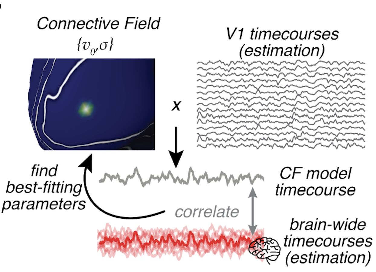

We have recently published some work with this method, and are planning on bringing out a lot more work based on this method. Our software that does prf fitting has also been adapted to fit connective field models. More on that soon.